
앙상블이 무엇인지, 배깅이 무엇인지 궁금하다면
Click ☞ https://joyfuls.tistory.com/61
Random Forest 알고리즘
- 여러 개의 결정 트리를 임의적으로 학습하는 앙상블의 배깅 유형
- 분류, 회귀 분석 모두 가능 (분류, 회귀 등에서 가장 많이 사용)
- 별도 튜닝(스케일 조정) 과정 없음
- 장점 : 단일 트리 모델 단점 보완(성능, 과대적합)
- 단점 : 대용량 데이터 셋으로 처리시간 증가
- 멀티코어 프로세스 이용 병렬처리 가능
- 배깅과의 차이점 : 배깅은 샘플 복원 추출 시 모든 설명변수 사용 but 랜덤포레스트는 a개의 설명변수만 복원 추출
- 랜덤포레스트는 일반적으로 배깅보다 성능이 우수
(설명변수가 많을 경우, 대체로 변수간 상관성이 높은 변수가 섞일 확률이 높은데 그 가능성을 제거하기 때문)
가장 적절한 트리(Tree) 개수와 설명변수 개수?
1) bootstrap의 수 m은 어느 정도로 커야할까?
: m이 100 이상이면 충분하지만 검정오차가 안정화될 만큼 큰 값을 사용 (400개 이상)
2) 랜덤포레스트의 설명변수 개수 a는 얼마가 적당할까?
: 전체 변수 개수가 p라면, 회귀트리는 1/3p, 분류트리는 p의 제곱급 = sqrt(p)
이는 주로 사용되는 개수일뿐, 실제로는 이 값의 주변 값을 확인해 볼 필요가 있다.
변수간 상관성에 따라 최적의 a값이 다를 수 있기 때문이다.
< 실습한 내용>
1. RandomForest Classifier
2. RandomForest Regressor
1. RandomForest 분류기 (분류 예측 모델)
"""
RandomForest Classifier
"""
from sklearn.ensemble import RandomForestClassifier #분류트리(모델)
from sklearn.model_selection import train_test_split # train/test
from sklearn.datasets import load_wine # dataset
from sklearn.metrics import accuracy_score, confusion_matrix # 평가 : 분류정확도
from sklearn.metrics import classification_report # 평가 : 정확률, 재현율, f1_score
# 1. dataset loading
X, y = load_wine(return_X_y = True)
X.shape # (178, 13)
y.shape # (178,)
y # 0, 1, 2 세개의 도메인 가지고 있음
# 2. train/test
X_train, X_test, y_train, y_test = train_test_split(X, y, test_size=0.3)
# 3. RF model 생성
model = RandomForestClassifier() # 분류 트리(default) 객체 생성
model.fit(X=X_train, y=y_train)
# 4. model 평가
y_pred = model.predict(X = X_test)
y_true = y_test
acc = accuracy_score(y_true, y_pred)
print('분류정확도 =', acc)
# 분류정확도 = 0.9814814814814815
con_mat = confusion_matrix(y_true, y_pred)
con_mat
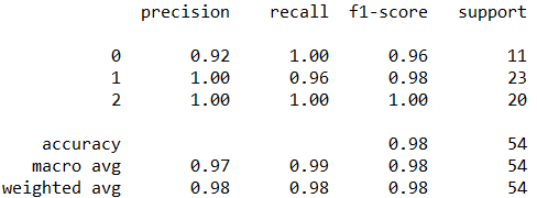
report = classification_report(y_true, y_pred)
report
###########################
### RF model tuning
###########################
help(RandomForestClassifier)
'''
n_estimators=10 : raw sampling 수
min_samples_split=2 : 설명변수 개수
'''
from math import sqrt
sqrt(13) # # 3.605551275463989 # 3 ~ 4 => 설명변수 개수
model = RandomForestClassifier(n_estimators=400, min_samples_split=3)
# 파라미터를 조절함으로써 좀 더 개선된 모델 생성이 가능하다
model.fit(X=X_train, y=y_train)
y_pred = model.predict(X = X_test)
y_true = y_test
acc = accuracy_score(y_true, y_pred)
print('분류정확도 =', acc)
# 분류정확도 = 1.0
2. RandomForest 회귀예측기 (값 예측 모델)
"""
RandomForest Regressor
"""
from sklearn.ensemble import RandomForestRegressor # 회귀트리(모델)
from sklearn.model_selection import train_test_split # train/test
from sklearn.datasets import fetch_california_housing, load_boston # dataset
from sklearn.metrics import mean_squared_error # 평균제곱오차
# 1. dataset loading
X, y = fetch_california_housing(return_X_y=True)
X.shape # (20640, 8)
y.shape # (20640,)
# 관측치 10개 확인
X[:10, :] # x변수 정규화
y[:10]
# [4.526, 3.585, 3.521, 3.413, 3.422, 2.697, 2.992, 2.414, 2.267, 2.611]
# 2. 정규화
import numpy as np
y = np.log(y)
y[:10]
# [1.50983855, 1.27675847, 1.25874504, 1.22759167, 1.23022518, 0.99214004, 1.09594206, 0.88128512, 0.81845737, 0.95973329]
y[:100]
# 3. model 생성
model = RandomForestRegressor()
model.fit(X = X, y = y)
y_pred = model.predict(X)
y_true = y
# 4. model 평가 : 평균제곱오차 - 작을수록 정확
mse = mean_squared_error(y_true, y_pred)
print('mse=', mse)
# mse= 0.010559916306010872
y_true[:10]
y_pred[:10]
# 상관관계 - 높을수록 정확
import pandas as pd
df = pd.DataFrame({'y_true':y_true, 'y_pred':y_pred})
cor = df['y_true'].corr(df['y_pred'])
cor # 0.984192504413277
######################
### load_boston
######################
# 1. dataset load
X, y = load_boston(return_X_y=True)
X.shape # (506, 13)
boston = load_boston()
X = boston.data
y = boston.target
colnames = boston.feature_names # 13개 칼럼 이름 가져올때
colnames
# ['CRIM', 'ZN', 'INDUS', 'CHAS', 'NOX', 'RM', 'AGE', 'DIS', 'RAD', 'TAX', 'PTRATIO', 'B', 'LSTAT']
# 2. train/test split
x_train, x_test, y_train, y_test = train_test_split(X, y, test_size=0.3)
x_train.shape # (354, 13)
# 3. model
model = RandomForestRegressor(n_estimators=400, min_samples_split=3)
model.fit(X = x_train, y = y_train)
# 4. model의 중요변수
imp = model.feature_importances_
imp
# [0.03380536, 0.00116905, 0.00627223, 0.00086973, 0.02241953, 0.2999559 , 0.01390804, 0.05426967, 0.0035352 , 0.01679749, 0.01656497, 0.01210188, 0.51833097]
len(imp) # 13 => 13개 칼럼들
colnames
import matplotlib.pyplot as plt
plt.barh(range(13), imp) # (x, y) # 중요도 (y에 얼마나 영향을 미치는지)
plt.yticks(range(13), colnames) # 축 이름

Example
'Python 과 머신러닝 > III. 머신러닝 모델' 카테고리의 다른 글
| [Python 머신러닝] 8장. 군집분석 (Cluster Analysis) (0) | 2019.10.29 |
|---|---|
| [Python 머신러닝] 7장. 앙상블 (Ensemble) - (3) XGBoost (0) | 2019.10.28 |
| [Python 머신러닝] 7장. 앙상블 (Ensemble) - (1) 앙상블의 개념 (0) | 2019.10.25 |
| [Python 머신러닝] 6장. 분류 (Classification) (w/ scikit-learn) (0) | 2019.10.25 |
| [Python 머신러닝] 5장. 회귀분석 - (2) 로지스틱 회귀분석 (0) | 2019.10.24 |


댓글