
앙상블이 무엇인지, 부스팅이 무엇인지 궁금하다면
Click ☞ https://joyfuls.tistory.com/61
XGBoost 알고리즘
- 여러 개의 결정 트리를 임의적으로 학습하는 앙상블의 부스팅 유형
- 순차적 학습 방법 => 약한 분류기를 강한 분류기로 만듦
- 분류정확도는 우수하나, Outlier에 취약함
- '캐글' 도전 데이터 과학자에서 5년 연속 1위한 알고리즘 (캐글 : https://www.kaggle.com/)
- 다양한 속성으로 모델 생성
• objective = "binary:logistic“, “reg:linear”“, “multi:softmax” : 이항 / 연속 / 다항
• max_depth = 2 : tree 구조가 간단한 경우 : 2
• nthread = 2 : cpu 사용 수 : 2
• nrounds = 2 : 실제값과 예측값의 차이를 줄이기 위한 반복학습 횟수
• eta = 1 : 학습률을 제어하는 변수(Default: 0.3), 오버 피팅을 방지
XGBoost 패키지 설치
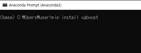
- 'Anaconda Prompt'에서 'pip install xgboost' 입력
- 외부 라이브러리 설치이기 때문에 아타콘다 프롬프트에서 다운 받는 것 (파이참 내부에서 불가능)
- 인터넷이 연결되어 있고 시스템이 정상적이라면 다음과 같이 설치가 진행됨
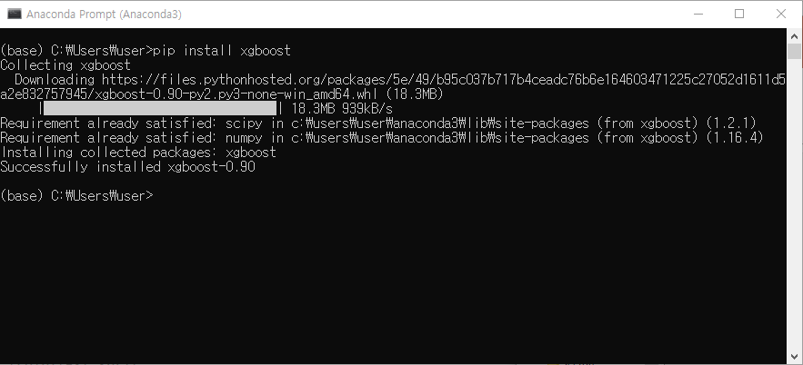
- 패키지 설치가 완료되면 'Spyder'에서 import해서 사용 가능
- 제거하려면 아나콘다 프롬프트에서 'pip uninstall xgboost' 입력하면 패키지 제거됨
<실습한 내용>
1. XGBoost 분류
2. XGBoost 회귀예측
3. XGBoost 실습(1) (fetch california housing 데이터)
4. XGBoost 실습(2) (동파유무 데이터)
1. XGBoost 분류
from xgboost import XGBClassifier # model
from xgboost import plot_importance # 중요변수 시각화
from sklearn.model_selection import train_test_split # train/test
from sklearn.metrics import accuracy_score, confusion_matrix, classification_report # model 평가
import pandas as pd
# 1. dataset load
iris = pd.read_csv("../data/iris.csv")
iris.info()
cols = list(iris.columns)
cols
col_x = cols[:4]
col_y = cols[-1]
col_x # ['Sepal.Length', 'Sepal.Width', 'Petal.Length', 'Petal.Width']
col_y # 'Species'
# 2. train/test split (8:2)
iris_train, iris_test = train_test_split(iris, test_size=0.2, random_state=123)
iris_train.shape # (120, 5)
iris_test.shape # (30, 5)
# 3. model 생성
model = XGBClassifier()
model.fit(X=iris_train[col_x], y=iris_train[col_y])
model
'''
n_estimators=100 : 트리를 100개 사용
min_child_weight=1 : 노드를 분할할때 사용한 설명변수 개수
objective='multi:softprob' : 다항분류(자동으로 설정됨)
'''
# 4. 중요변수 확인/시각화 : y에 영향을 미치는 변수
fscore = model.get_booster().get_fscore()
fscore
'''
{'Petal.Length': 282,
'Petal.Width': 235,
'Sepal.Length': 92,
'Sepal.Width': 66}
'''
plot_importance(model)

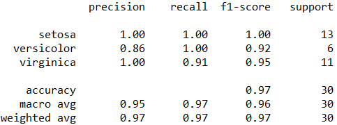
# 5. model 평가
y_pred = model.predict(iris_test[col_x]) # 예측치
y_true = iris_test[col_y] # 정답
acc = accuracy_score(y_true, y_pred)
acc # 0.9666666666666667
con_mat = confusion_matrix(y_true, y_pred)
con_mat
report = classification_report(y_true, y_pred)
print(report)
2. XGBoost 회귀예측
from xgboost import XGBRegressor # 회귀트리 모델
from xgboost import plot_importance # 중요변수 시각화
from sklearn.datasets import load_boston # dataset
from sklearn.model_selection import train_test_split
from sklearn.metrics import mean_absolute_error, mean_squared_error
# 1. data loading
boston = load_boston()
X = boston.data
y = boston.target
col_names = boston.feature_names
X.shape # (506, 13) # 13개의 칼럼
col_names # 칼럼이름
y.shape # (506,)
y # 수치 데이터 => 회귀
# 2. train/test split
x_train, x_test, y_train, y_test = train_test_split(X, y, test_size = 0.3)
x_train.shape # (354, 13)
x_test.shape # (152, 13)
# 3. model
model = XGBRegressor()
model.fit(x_train, y_train)
model
# objective='reg:linear' => 회귀트리
# 4. 중요변수 시각화
import matplotlib.pyplot as plt
plot_importance(model)
plt.yticks(range(13), col_names)
plt.show()

# 5. model 평가
y_pred = model.predict(x_test)
y_true = y_test
mae = mean_absolute_error(y_true, y_pred)
mae # 2.3400885707453676
mse = mean_squared_error(y_true, y_pred)
mse # 12.75553963355965
3. XGBoost 실습(1) (fetch california housing 데이터)
from xgboost import XGBRegressor
from xgboost import plot_importance, plot_tree
from sklearn.datasets import fetch_california_housing # dataset
from sklearn.metrics import mean_squared_error
from sklearn.model_selection import train_test_split
housing = fetch_california_housing()
X = housing.data
y = housing.target
col_names = housing.feature_names
X.shape # (20640, 8)
X
y.shape # (20640,)
y[:10]
y[-10:]
type(X) # numpy.ndarray => 함수활용 가능
type(y) # numpy.ndarray
import numpy as np
y.mean() # 2.068558169089147
y = np.log(y) # log를 통해 정규화 => 특이값, 편향을 제거하는 것이 목적
y.mean() # 0.5719587205516943
y[:10]
##########################
### numpy -> DataFrame
##########################
# 필요에 따라 numpy와 DF 형태를 왔다갔다 바꾸면서 각 형태에서 제공하지않는 부분을 서로 보완할 수 있음
import pandas as pd
X_df = pd.DataFrame(X, columns = col_names) # X를 행렬로 표현, 칼럼 이름 설정
X_df
# train_test_split - test_size 생략시, 75:25 가 default
x_train, x_test, y_train, y_test = train_test_split(X_df, y) # test_size = 0.25
x_train.shape # (15480, 8)
type(x_train) # DataFrame
y_train.shape # (15480,)
type(y_train) # numpy.ndarray
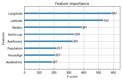
# model 생성
model = XGBRegressor(n_estimators=400) # 트리의 개수 400개로 모델 생성
model.fit(x_train, y_train)
model
# objective='reg:linear'
# 중요변수 시각화
plot_importance(model)
# model 평가
y_pred = model.predict(x_test)
y_true = y_test
mse = mean_squared_error(y_true, y_pred)
mse # 0.05036776284314333
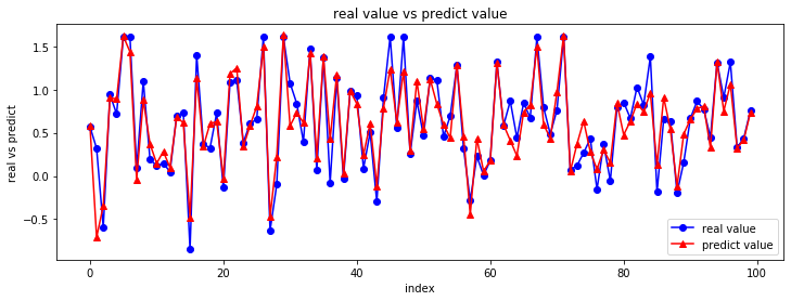
# y_true vs y_pred (시각화해서 비교)
import matplotlib.pyplot as plt
# y_true.shape # (5160,) : 5160개의 데이터 => 많으니까 100개만 출력 시도
fig = plt.figure( figsize = (12, 4) )
chart = fig.add_subplot(1,1,1)
chart.plot(y_true[:100], marker='o', color='blue', label='real value')
chart.plot(y_pred[:100], marker='^', color='red', label='predict value')
chart.set_title('real value vs predict value')
plt.xlabel('index')
plt.ylabel('real vs predict')
plt.legend(loc = 'best')
# 위에 블럭 실행
4. XGBoost 실습(2) (동파유무 데이터)
"""
수도사업소 주관 - big 콘테스트 dataset
- 동파유무 분류를 위한 dataset
- 동파유무에 영향을 미치는 중요변수 분석
"""
import pandas as pd # csv file
from xgboost import XGBClassifier # 분류트리
from sklearn.model_selection import train_test_split
from xgboost import plot_importance
from sklearn.metrics import accuracy_score, confusion_matrix, classification_report
# 한글 지원
from matplotlib import font_manager, rc
font_name = font_manager.FontProperties(fname="c:/Windows/Fonts/malgun.ttf").get_name()
rc('font', family=font_name)
from matplotlib import pyplot as plt # 시각화
import time # 시간 측정
# 1. dataset load
freeze = pd.read_csv("../data/freeze_dataset.csv", encoding="ms949") # 보통 "utf-9" 아니면 "ms949"
freeze.info()
'''
RangeIndex: 37089 entries, 0 to 37088
Data columns (total 95 columns):
'''
# 칼럼명 공백 -> "_"
freeze.columns = freeze.columns.str.replace(" ", "_")
freeze.info()
# y변수 빈도수
freeze['동파유무'].value_counts()
'''
0.0 34130 : 동파 무 = 0 : 92%
1.0 2959 : 동파 유 = 1 : 8%
'''
34130 / 37089
# 소요 시간 (현재시간 측정 => 끝날 때 측정한 시간)
chktime = time.time() # 현재 시간
# 2. train/test split : 60 vs 40
freeze_train, freeze_test = train_test_split(freeze, test_size = 0.4)
freeze_train.shape # (22253, 95)
freeze_test.shape # (14836, 95)
cols = list(freeze.columns)
col_x = cols[1:]
col_y = cols[0]
# 3. model 생성
model = XGBClassifier(n_estimators=500)
model.fit(freeze_train[col_x], freeze_train[col_y])
model # 데이터가 크면 모델 생성시 소요시간 증가
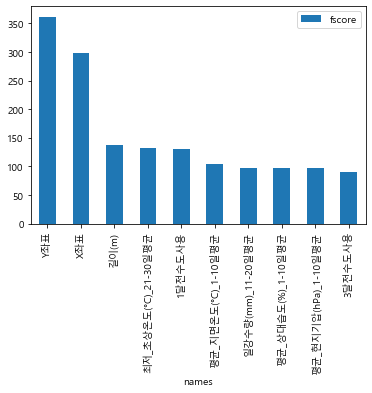
# 4. 중요변수 fscore
fscore = model.get_booster().get_fscore()
fscore
len(fscore) # 59
sorted(fscore)
# 내림차순 정렬 key
names = sorted(fscore, key=fscore.get, reverse=True)
names
# fscore 내림차순 정렬
score = [fscore[key] for key in names]
score
fscore_df = pd.DataFrame({'names':names, 'fscore':score})
fscore_df.info()
# 중요변수 top10 시각화
new_fscore_df = fscore_df.set_index('names') # index 변경
new_fscore_df.iloc[:10, :].plot(kind='bar')
# 중요변수 시각화
# plot_importance(model)
# 5. model 평가
y_pred = model.predict(freeze_test[col_x])
y_true = freeze_test[col_y]
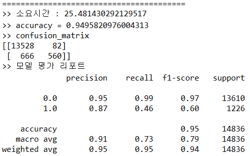
curr_time = time.time() - chktime
print('='*40)
print('>> 소요시간 :', curr_time)
acc = accuracy_score(y_true, y_pred)
print(">> accuracy =", acc) # accuracy = 0.9524130493394446
con_mat = confusion_matrix(y_true, y_pred)
print(">> confusion_matrix")
print(con_mat)
'''
[[13600 75] => 0인 경우
[ 631 530]] => 1인 경우
'''
# accuracy로 볼 때는 상당히 높은 정확률을 보이지만
# 0에 대한 정밀도와 재현율, 1에 대한 정밀도와 재현율에서 크게 차이가 있다.
# 여기서 모델의 예측력은 f1-score로 판단
report = classification_report(y_true, y_pred)
print(">> 모델 평가 리포트")
print(report)
Example
'Python 과 머신러닝 > III. 머신러닝 모델' 카테고리의 다른 글
| [Python 머신러닝] 9장. 추천시스템 (Recommendation System) (0) | 2019.10.30 |
|---|---|
| [Python 머신러닝] 8장. 군집분석 (Cluster Analysis) (0) | 2019.10.29 |
| [Python 머신러닝] 7장. 앙상블 (Ensemble) - (2) RandomForest (0) | 2019.10.25 |
| [Python 머신러닝] 7장. 앙상블 (Ensemble) - (1) 앙상블의 개념 (0) | 2019.10.25 |
| [Python 머신러닝] 6장. 분류 (Classification) (w/ scikit-learn) (1) | 2019.10.25 |


댓글