
로지스틱 회귀분석이란?
선형회귀로 풀 수 없는 문제가 있다면?
- 로지스틱 회귀는 두 개의 카테고리로 분류되는 범주형 데이터를 예측할 때 적합하다.
- ex. 합격/불합격, 높음/낮음, 정답/오답 등
1) 오즈비 vs 로짓변환
오즈비(Odds ratio) : 0(실패)에 대한 1(성공)의 비율 ( 0 : no, 1 : yes )
- no인 상태와 비교하여 yes가 얼마나 높은지 낮은지 정량화한 것
- 오즈비 = p (success) / 1-p (fail)
- p : y=1이 나올 확률, 1-p : y=1의 여사건
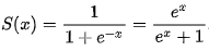
로짓(logit) 변환
- 오즈비에 log 함수 적용한 것
- 로짓 = log( p / 1-p )
=> 로짓을 대상으로 회귀분석을 적용한 것이 로지스틱 회귀분석(Logistic Regression Analysis)
2) 시그모이드 함수 (Sigmoid Function)
- 선형회귀만으로 해결이 안되던 문제, 어떤 값을 넣든 결과가 0~1 을 출력해야 하는 문제
> 기존의 가설의 결과를 0~1 범위로 나타낼 수 있는 시그모이드 함수 발견
<- 시그모이드 함수 (로지스틱 함수의 일종)
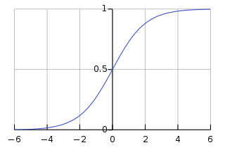
- 위 그래프처럼 0과 1 사이에 집약되어 있고 그 모양이 S 형태를 띄기 때문에 Sigmoid라는 이름이 붙는다.
- 합격/불합격을 분류한 데이터를 학습 > 시그모이드 함수 > x값을 넣으면 y 값은 0~1 사이의 확률로 예측됨
-----------------------------------------------< 실습 >-----------------------------------------------
"""
sklearn 로지스틱 회귀모델 생성
- y변수가 범주형인 경우
- 평가방법 : 분류정확도
"""
from sklearn.datasets import load_iris, load_breast_cancer # dataset
from sklearn.linear_model import LogisticRegression # 모델 생성
from sklearn.metrics import accuracy_score, confusion_matrix # 분류정확도, 교차분할표 : 모델 평가
###################
### 이항분류
###################
# 1. dataset loading
breast = load_breast_cancer()
breast
# 2. 변수 선택
breast_x = breast.data
breast_y = breast.target # 0 or 1 인 데이터
breast_x.shape # (569, 30)
breast_y.shape # (569,)
# 3. model 생성
model = LogisticRegression()
model.fit(X=breast_x, y=breast_y)
model.coef_ # 기울기
model.intercept_ # 절편
# 4. model 평가
y_pred = model.predict(breast_x)
y_pred
y_pred[:20]
breast_y[:20]
acc = accuracy_score(breast_y, y_pred)
print('accuracy =', acc)
# accuracy = 0.9595782073813708
# 정확도를 식으로 직접 구하는 방법
# confusion matrix
import pandas as pd
tab = pd.crosstab(breast_y, y_pred)
tab
'''
col_0 0 1
row_0
0 198 14
1 9 348
'''
acc = (tab.iloc[0,0] + tab.iloc[1,1]) / len(breast_y)
print('accuracy =', acc)
# accuracy = 0.9595782073813708
#####################
### 다항분류
#####################
# 1. dataset loading
X, y = load_iris(return_X_y=True) # X변수 y변수를 로드하면서 동시에 가져오겠다는 의미
X.shape # (150, 4) - 2차원
y.shape # (150,) - 1차원
y # 0, 1, 2 로 이루어진 다항분류 데이터
# 2. model 생성
help(LogisticRegression)
# solver = 'lbfgs'
# multi_class = 'multinomial'
model = LogisticRegression(random_state=0, solver ='lbfgs', multi_class='multinomial')
# random_state=0 : 실행할때마다 값이 달라지니 랜덤 효과 없애기 위해 설정
# solver ='lbfgs', multi_class='multinomial' : 다항분류를 위한 옵션
model.fit(X=X, y=y) # 학습수행
# 3. model 평가
# 예측치
y_pred = model.predict(X=X)
# 분류정확도
acc = accuracy_score(y, y_pred)
print('accuracy =', acc)
# accuracy = 0.9733333333333334
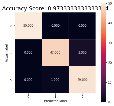
# confusion matrix
con_mat = confusion_matrix(y_true=y, y_pred=y_pred)
con_mat
'''
array([[50, 0, 0],
[ 0, 47, 3],
[ 0, 1, 49]], dtype=int64)
'''
acc = (con_mat[0,0] + con_mat[1,1] + con_mat[2,2])/len(y)
print('accuracy =', acc)
# accuracy = 0.9733333333333334
# 정확도를 heatmap으로 시각화하기
import seaborn as sn # heatmap - Accuracy Score
import matplotlib.pyplot as plt
# 아래를 블럭 실행하기
# confusion matrix heatmap
plt.figure(figsize=(6,6)) # chart size
sn.heatmap(con_mat, annot=True, fmt=".3f", linewidths=.5, square = True);# , cmap = 'Blues_r' : map »ö»ó
plt.ylabel('Actual label');
plt.xlabel('Predicted label');
all_sample_title = 'Accuracy Score: {0}'.format(acc)
plt.title(all_sample_title, size = 18)
plt.show()
----------------------------------------------- example -----------------------------------------------
'Python 과 머신러닝 > III. 머신러닝 모델' 카테고리의 다른 글
| [Python 머신러닝] 7장. 앙상블 (Ensemble) - (2) RandomForest (0) | 2019.10.25 |
|---|---|
| [Python 머신러닝] 7장. 앙상블 (Ensemble) - (1) 앙상블의 개념 (0) | 2019.10.25 |
| [Python 머신러닝] 6장. 분류 (Classification) (w/ scikit-learn) (1) | 2019.10.25 |
| [Python 머신러닝] 5장. 회귀분석 - (1) 선형 회귀분석 (1) | 2019.10.23 |
| [Python 머신러닝] 지도학습과 비지도학습 (0) | 2019.10.23 |


댓글